Hypothesis Test: Population Mean: Two Samples: Matched Pairs
Dataset: MatchedWeights (the name we shall give it because it does not have a name)
Source: MyLab Math (MLM)
1st Column: Reported Weights
2nd Column: Measured Weights
Description:
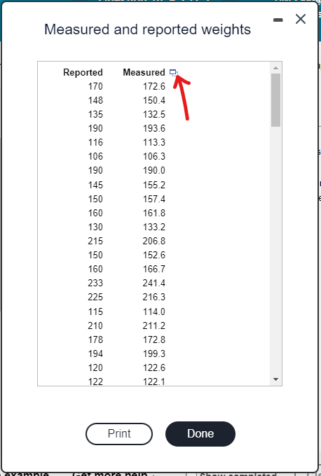
The data set gives the measured and reported weights (in pounds) of 127 female subjects.
Question:
Listed in the accompanying table are 127 measured and reported weights (lb) of female subjects.
Use the listed paired sample data, and assume that the samples are simple random samples and that the differences have a distribution that is approximately normal.
(a.) Use a 0.05 significance level to test the claim that for females, the measured weights tend to be higher than the reported weights.
In this example, μd is the mean value of the differences d for the population of all pairs of data, where each individual difference d is defined as the measured weight minus the reported weight.
What are the null and alternative hypotheses for the hypothesis test?
The difference is the: measured weights minus the reported weights.
Null Hypothesis: H0: μd = 0 (because the measured weights is assumed to be equal to the reported weights.)
Alternative Hypothesis: H1: μd > 0 (because the measured weights tend to be higher than the reported weights.)
(b.) Test the claim that the measured weights tend to be higher than the reported weights for females.
Use at least two approaches.
Interpret your results. This includes your decision and your conclusion.
Variable of both subjects: Weight
Unit of the variable(s): pounds
Sample Size for both subjects: 127
Sample: 127 American females in the year 2023 (the nationality and year are assumed.)
Population: All American females in the year 2023 (the nationality and year are assumed.)
Objectives:
(1.) Test the claim that the measured weights of 127 American females in year 2023 are higher than their reported weights using the Critical Value Method (Classical Approach).
(2.) Test the claim that the measured weights of 127 American females in year 2023 are higher than their reported weights using the P-Value (Probability-Value) Approach.
(3.) Test the claim that the measured weights of 127 American females in year 2023 are higher than their reported weights using the Confidence Interval Method.
(4.) Interpret the results.
(5.) Write the decision.
(6.) State the conclusion.
Parameter to test: Population Mean
Test: t-test
Direction of Test: Right-tailed test (because of the greater than symbol: > in the alternative hypothesis)
Reason for Test: The population standard deviation was not given.
Verify Requirements for Test
(1.) The sample data are matched pairs and equal sample size.
(2.) The matched pairs are simple random samples.
(3.) The sample size is large (at least a sample size of 30 for each pair).
(4.) The population from which the pairs of values were drawn is normally distributed.
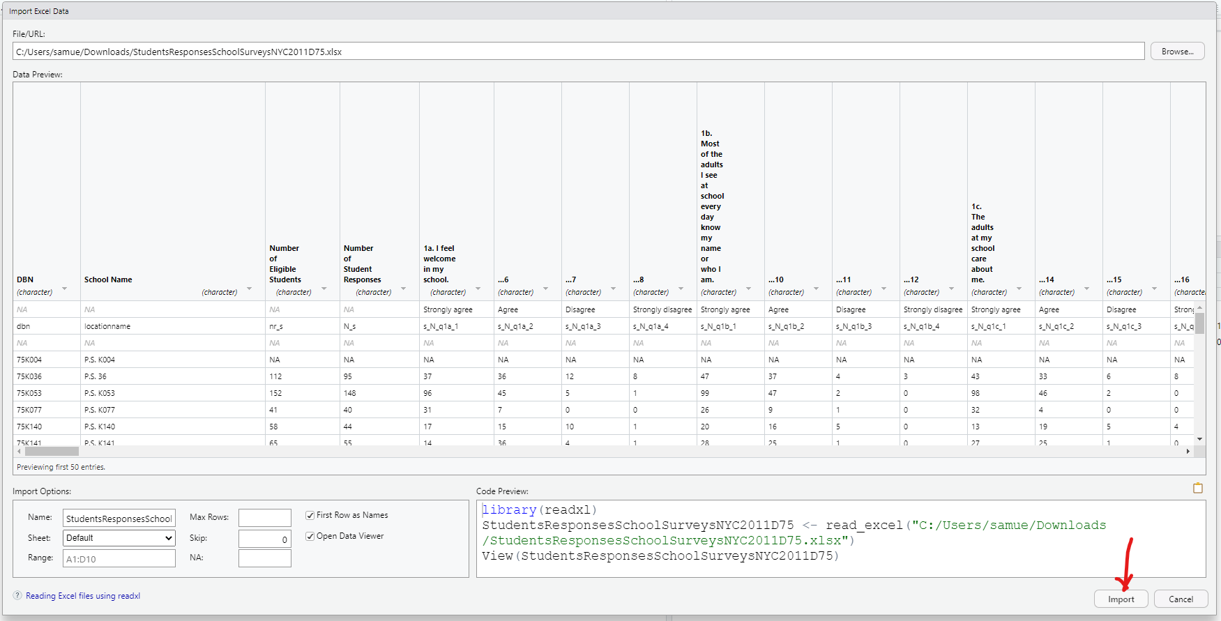
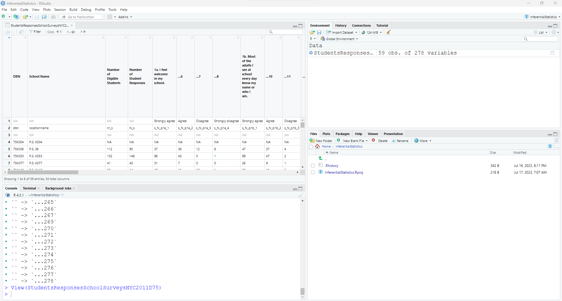
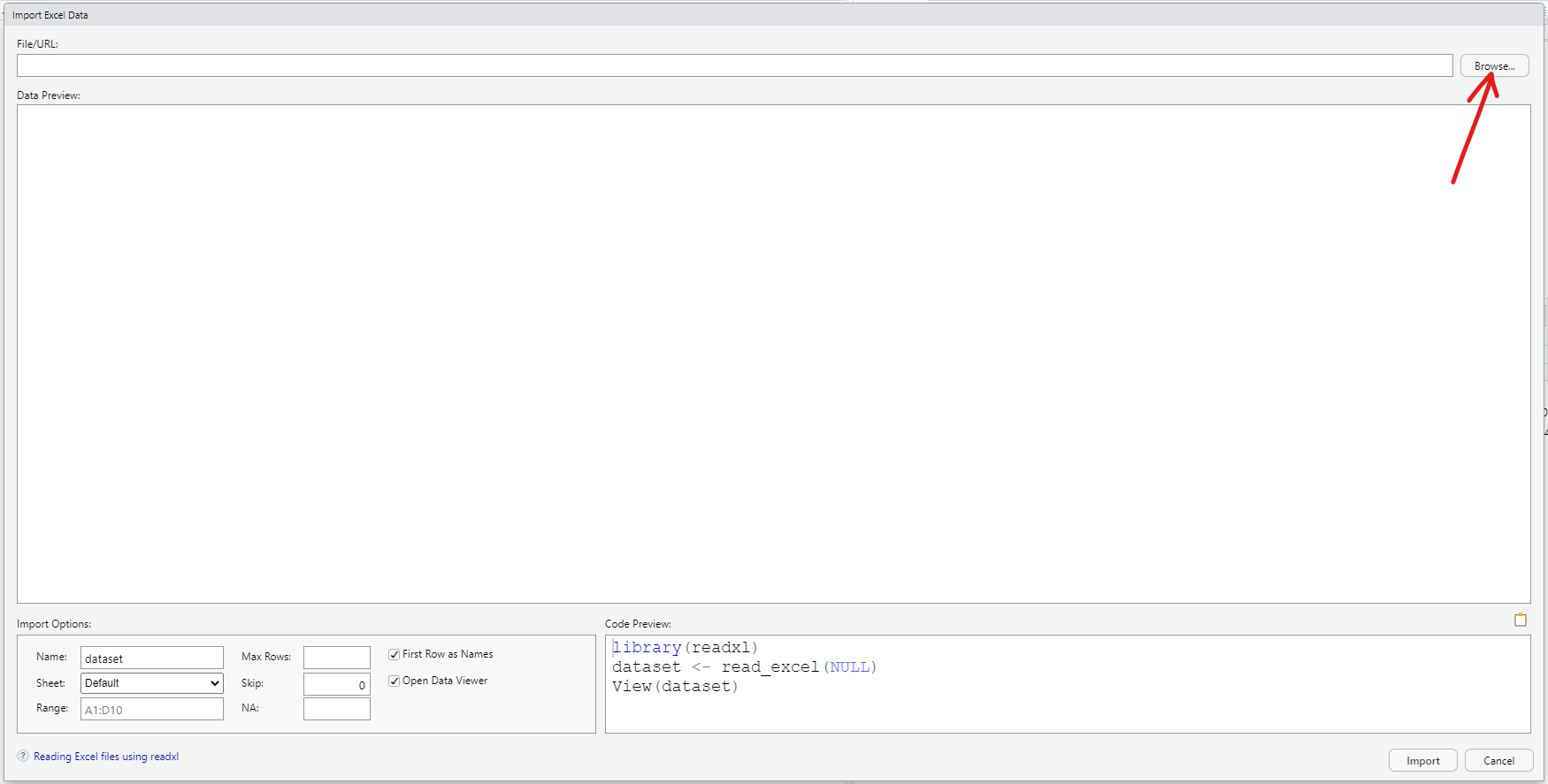
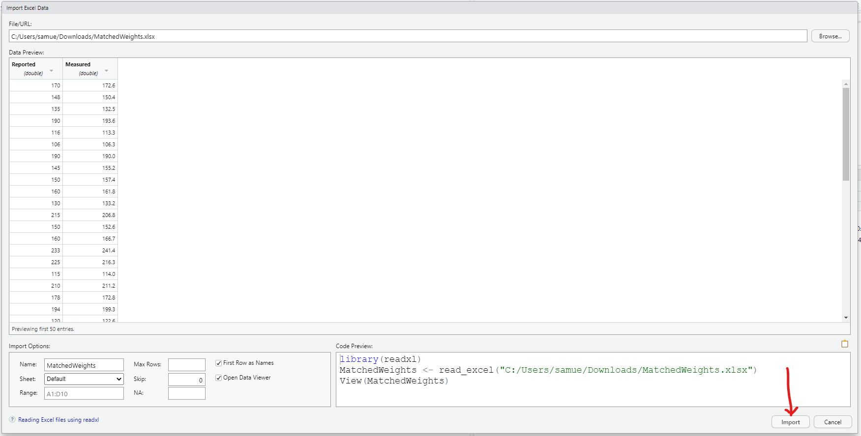
Download the dataset. Rename it to MatchedWeights


Import the dataset into RStudio


1st Approach: Critical Value (Classical) Approach
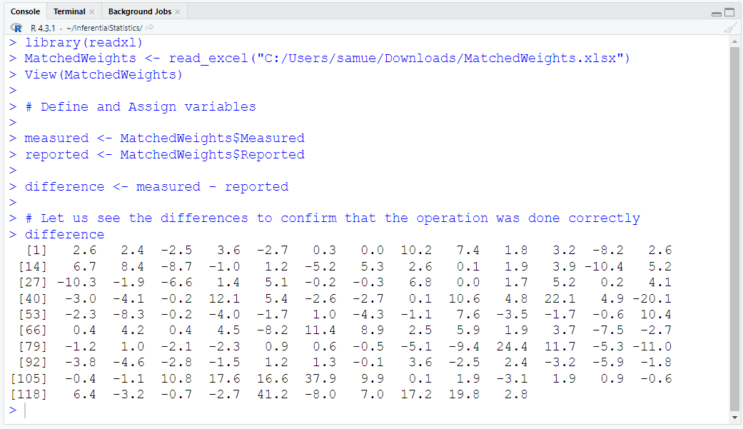
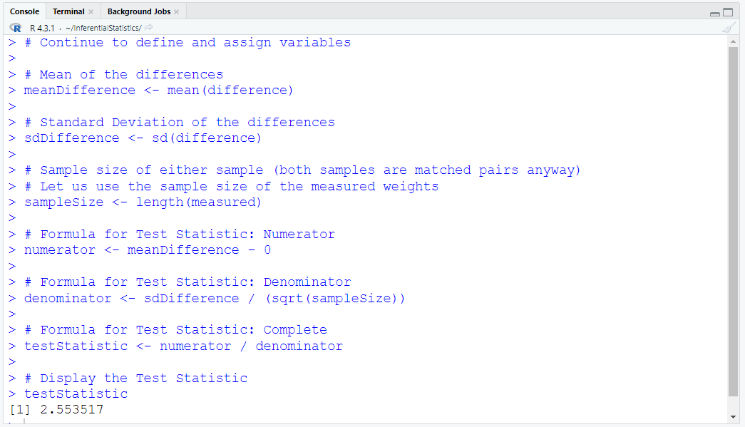
Define and Assign Variables. Use appropriate names for the variables.
$
t = \dfrac{\bar{x}_d - \mu_d}{\dfrac{s_d}{\sqrt{n}}} \\[7ex]
$
where:
$d$ is the differences for the paired sample data (difference between the measured weight and the reported weight)
$t$ is the t test statistic
$\bar{x}_d$ is the mean of the differences for the paired sample data
$s_d$ is the standard deviation of the differences for the paired sample data
$\mu_d$ is the mean value of the differences for the population of all the pairs of data
$n$ is the sample size of either sample (because of matched pair of samples)
Did you notice the:
(a.) exact value of the test statistic?
(b.) approximate value of the test statistic?
We have determined the test statistic
We need to determine the critical value of the t distribution.
The level of significance is 0.05 (given by the question)
The test is a Right-tailed test (because of the alternative hypothesis)
The degrees of freedom for a one-tailed right-tailed test is 1 less than the sample size (sample size − 1)
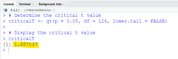
The qt() function is used to determine the critical t
For one-tailed left-tailed test; the qt() function is: qt(p = significanceLevel, df = sampleSize − 1, lower.tail = TRUE) or
qt(p = significanceLevel, df = sampleSize) (because the lower tail is left-tailed by default, so omitting that argument treats the lower tail as left-tailed)
If we want a right-tailed test, then we set the lower tail to the Boolean value of FALSE
For one-tailed right-tailed test; the qt() function is: qt(p = significanceLevel, df = sampleSize − 1, lower.tail = FALSE)
For two-tailed test; the qt() function is: qt(p = significanceLevel / 2, df = sampleSize − 2, lower.tail = FALSE)
So, the code we shall use is: qt(p = 0.05, df = 126, lower.tail = FALSE)
Did you notice the:
(a.) exact value of the test statistic?
(b.) approximate value of the test statistic?
Interpretation:
Critical Value Method for Right-tailed test:
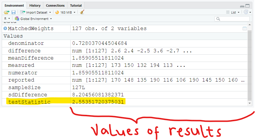
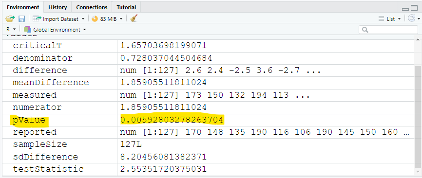
The t test statistic is: 2.55351720375031
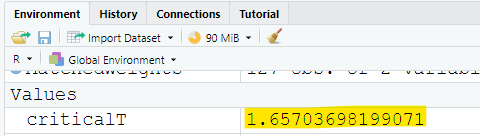
The critical t value is: 1.65703698199071
The test statistic is greater than the critical value
This implies that the test statistic falls in the critical region
Decision: Reject the null hypothesis
Conclusion: There is sufficient evidence to support the claim that measured weights tend to be higher than the reported weights.
2nd Approach: Probability-Value (P-Value) Approach
Let us determine the probability that the critical value is greater than the test statistic
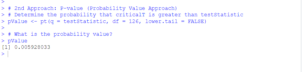
To determine this probability, we shall use the pt() function
For one-tailed left-tailed test; P(criticalT < −testStatistic) is the pt() function, and is: pt(p = −1 * testStatistic, df = sampleSize − 1, lower.tail = TRUE) or
pt(p = -1 * testStatistic, df = sampleSize) (because the lower tail is left-tailed by default, so omitting that argument treats the lower tail as left-tailed)
If we want a right-tailed test, then we set the lower tail to the Boolean value of FALSE
For one-tailed right-tailed test; P(criticalT > testStatistic) is the pt() function, and is: pt(p = testStatistic, df = sampleSize − 1, lower.tail = FALSE)
For two-tailed test; [P(criticalT < −testStatistic) + P(criticalT > testStatistic)] is the pt() function, and is: pt(p = *testStatistic*, df = sampleSize − 2, lower.tail = FALSE)
So, the code we shall use is: pt(q = testStatistic, df = 126, lower.tail = FALSE)
Did you notice the:
(a.) exact value of the probability value?
(b.) approximate value of the probability value?
Interpretation:
Probability Value Method for Right-tailed test:
The significance level is: 0.05
The probability value is: 0.00592803278263704
The probability value is less than the significance level
Decision: Reject the null hypothesis
Conclusion: There is sufficient evidence to support the claim that measured weights tend to be higher than the reported weights.
3rd Approach: Confidence Interval Approach
Define and Assign Variables. Use appropriate names for the variables.
$
CL = 1 - \alpha ...one-tailed\;\;test \\[3ex]
CL = 1 - 0.05 \\[3ex]
CL = 0.95 = 95\% \\[3ex]
E = t_{\dfrac{\alpha}{2}} = \dfrac{s_d}{\sqrt{n}} \\[5ex]
\underline{Confidence\;\;Interval} \\[3ex]
\bar{x}_d - E \lt \mu_d \lt \bar{x}_d + E \\[3ex]
$
where:
$\alpha$ is the significance level
$CL$ is the confidence level
$E$ is the margin of error
$t_{\dfrac{\alpha}{2}}$ is the critical t value
$\bar{x}_d - E$ is the lower bound of the confidence interval
$\bar{x}_d + E$ is the upper bound of the confidence interval
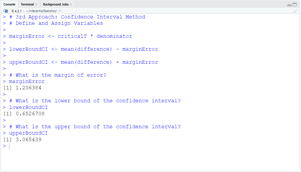
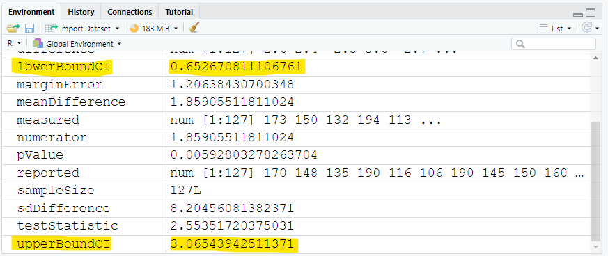
The 95% confidence interval is: (0.652670811106761, 3.06543942511371)
The lower bound of the confidence interval is: 0.652670811106761 pounds
The lower bound is greater than 0
The upper bound of the confidence interval is: 3.06543942511371 pounds
The upper bound is also greater than 0
The confidence interval does not contain 0.
Both bounds are positive. Therefore, it is likely that the mean of the differences is always greater than 0.
Decision: Reject the null hypothesis
Conclusion: There is sufficient evidence to support the claim that measured weights tend to be higher than the reported weights.